

Polynomials, those seemingly simple algebraic expressions, hold within them a universe of complexity and beauty. From the most basic linear equation to the most intricate higher-order curve, polynomials serve as fundamental building blocks in mathematics, physics, engineering, and countless other fields. Their ability to model diverse phenomena, predict trends, and solve complex problems makes them indispensable tools in the modern world.

Polynomial Vector Spaces: A Playground of Abstraction
One of the most powerful ways to understand polynomials is through the lens of linear algebra. Consider the set of all polynomials with real coefficients, up to a certain degree ‘n’. We can treat this set, denoted as Pn, as a vector space. This means we can add polynomials together and multiply them by scalar values, and the result will still be a polynomial within the same set. This seemingly simple concept opens up a whole world of possibilities for applying the tools and techniques of linear algebra to the study of polynomials.
Imagine each polynomial as a vector in an abstract space. The operations of addition and scalar multiplication then become geometric transformations within this space. We can define concepts like linear independence, basis, and dimension for these polynomial vector spaces, allowing us to analyze and manipulate polynomials in a more structured and efficient manner.
For instance, the set of all polynomials of degree at most 2 (P2) forms a vector space. A basis for this space could be 1, t, t2, meaning any polynomial in P2 can be expressed as a linear combination of these three basis vectors. This representation allows us to perform operations like differentiation and integration in a more streamlined way, as we can simply operate on the coefficients of the basis vectors.
Moreover, we can define linear transformations between polynomial vector spaces. These transformations map polynomials from one space to another while preserving the linear structure. Examples of such transformations include differentiation, integration, and evaluation at a specific point. Studying these transformations provides insights into the relationships between different polynomial spaces and allows us to solve problems involving polynomials in a more general and abstract setting.
The concept of eigenvalues and eigenvectors, so crucial in linear algebra, also finds application in polynomial vector spaces. An eigenvector of a linear transformation is a polynomial that, when transformed, remains a scalar multiple of itself. The corresponding eigenvalue represents the scaling factor. Finding eigenvalues and eigenvectors of polynomial transformations can reveal important properties of the transformation and the polynomial space itself.
For example, consider the differentiation operator acting on the space of polynomials. The eigenvectors of this operator are exponential functions, and the corresponding eigenvalues are the frequencies of those exponential functions. This connection between differentiation and exponential functions highlights the profound interplay between linear algebra and calculus within the context of polynomial vector spaces.
Understanding polynomial vector spaces provides a powerful framework for analyzing and manipulating polynomials in a more abstract and general way. It allows us to leverage the tools and techniques of linear algebra to solve problems involving polynomials and gain deeper insights into their properties.
Approximating with Grace: Exploring Function Behavior Through Ratios

Beyond their theoretical elegance, polynomials play a critical role in approximation theory. Often, we encounter functions that are too complex to handle directly, whether due to their intricate form or the lack of an explicit formula. In such cases, we can approximate these functions using polynomials. The idea is to find a polynomial that closely matches the behavior of the original function over a certain interval.
There are various techniques for polynomial approximation, each with its own strengths and weaknesses. Taylor polynomials provide a local approximation of a function around a specific point. They are based on the derivatives of the function at that point and become more accurate as we include higher-order terms. However, Taylor polynomials may not be accurate over a large interval, especially if the function exhibits rapid oscillations or singularities.
Chebyshev polynomials, on the other hand, are designed to minimize the maximum error over a given interval. They are particularly useful for approximating functions that are smooth and well-behaved. Chebyshev approximation often provides a more uniform and accurate approximation compared to Taylor polynomials.
The effectiveness of a polynomial approximation can be quantified by analyzing the error between the original function and the approximating polynomial. This error can be measured in various ways, such as the maximum absolute error or the root-mean-square error. By minimizing the error, we can obtain a polynomial that provides a good representation of the original function.
The image depicts a plot of the ratio of an exact solution, G(p)(t), to an approximate solution, G(p),N(t). Analyzing this ratio is crucial to understanding the accuracy and convergence of the approximation. Ideally, this ratio should be close to 1 over the entire interval of interest. Deviations from 1 indicate the presence of error in the approximation.
When the ratio oscillates around 1, it suggests that the approximation is capturing the general trend of the function but may not be accurate at specific points. Large deviations from 1 indicate significant errors in the approximation, possibly due to the choice of polynomial degree or the approximation method used.
By analyzing the behavior of this ratio, we can identify regions where the approximation is poor and refine the approximation method accordingly. This might involve increasing the degree of the polynomial, using a different approximation technique, or subdividing the interval into smaller subintervals.
In practical applications, polynomial approximation is used extensively in numerical analysis, computer graphics, and data fitting. It allows us to represent complex functions with simpler, more manageable expressions, enabling us to perform calculations, visualize data, and build predictive models.
For example, in computer graphics, polynomial curves are used to represent smooth shapes and surfaces. These curves are defined by a set of control points, and the polynomial is chosen to interpolate or approximate these points. By adjusting the control points, we can manipulate the shape of the curve and create visually appealing designs.
In data fitting, polynomial regression is used to find a polynomial that best fits a set of data points. This technique is used to model relationships between variables, predict future values, and identify trends in data.
The ability to approximate functions with polynomials is a powerful tool that allows us to simplify complex problems and gain insights into the behavior of functions. By carefully choosing the approximation method and analyzing the error, we can obtain accurate and reliable approximations that are useful in a wide range of applications.
In conclusion, polynomials, viewed through the lens of vector spaces and approximation techniques, are far more than just algebraic expressions. They are powerful tools for modeling, analyzing, and understanding the world around us. Their versatility and adaptability make them indispensable in various fields, from mathematics and physics to engineering and computer science. The deeper we delve into their properties and applications, the more we appreciate their elegance and power.
If you are searching about Plot of the ratio G (p) (t)/G (p),N (t), where G (p) is the exact you’ve came to the right page. We have 5 Images about Plot of the ratio G (p) (t)/G (p),N (t), where G (p) is the exact like Plot of the ratio G (p) (t)/G (p),N (t), where G (p) is the exact, Solved Show that n (t) = -g'(t)I + f'(t)j and -n(t) = g'(t)i | Chegg.com and also Solved N-IDT P2 a. Show that n(t) = – g'(t)i + f(t)j and – | Chegg.com. Read more:
Plot Of The Ratio G (p) (t)/G (p),N (t), Where G (p) Is The Exact
www.researchgate.net
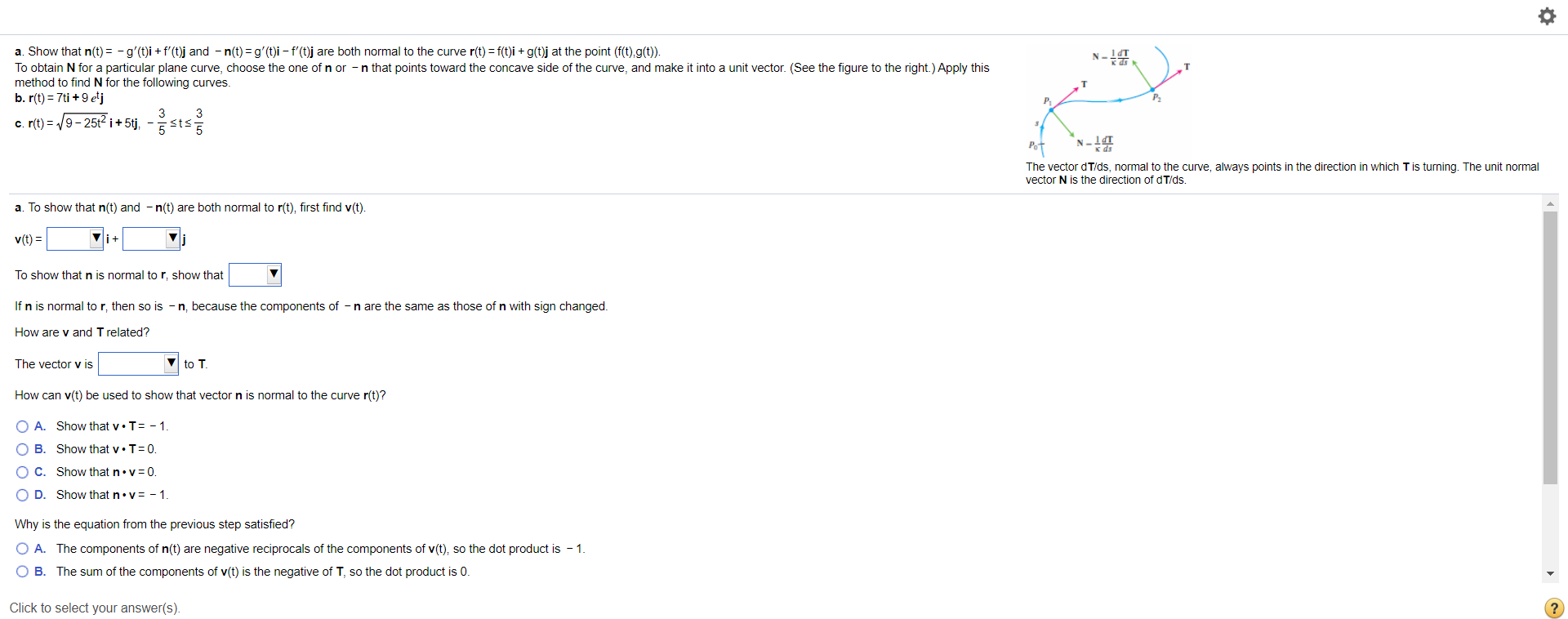
Solved N- A. Show That N(t)= – G'(t)i + F'(t)j And – N(t)=g' | Chegg.com
www.chegg.com
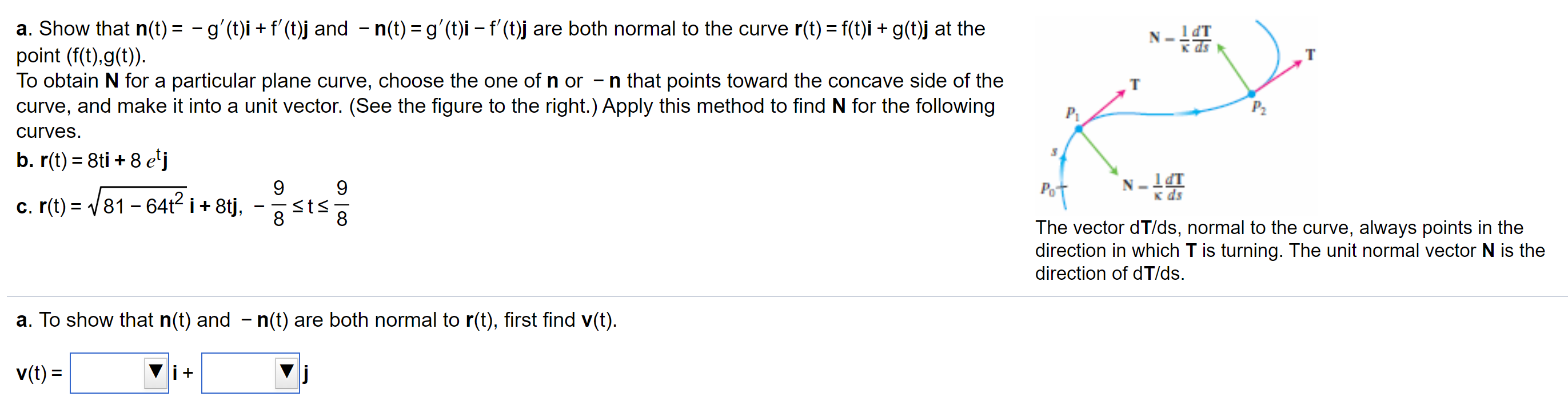
Solved N-IDT P2 A. Show That N(t) = – G'(t)i + F(t)j And – | Chegg.com
www.chegg.com
idt
Solved Show That N (t) = -g'(t)I + F'(t)j And -n(t) = G'(t)i | Chegg.com

www.chegg.com
show solved transcribed problem text been has
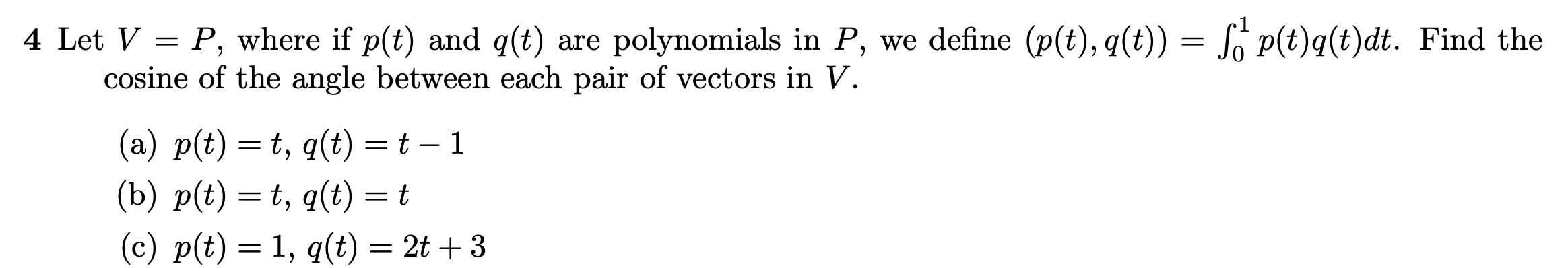
Solved 4 Let V = P, Where If P(t) And G(t) Are Polynomials | Chegg.com
www.chegg.com
Solved n-idt p2 a. show that n(t) =. Solved n- a. show that n(t)=. Show solved transcribed problem text been has
Gallery for p to the g to the n to the t Show solved transcribed problem text been has


